HX-DEAL Tutorial
In this tutorial, we will explain how to:
More information and sample data
[Link, Data] Raval S, Sarpe V, Hepburn M, Crowder DA, Zhang T, Viner R, Schriemer DC, Improving Spectral Validation Rates in Hydrogen-Deuterium Exchange Data Analysis. Anal Chem, 93(9):4246-4254(2021)
Create Project
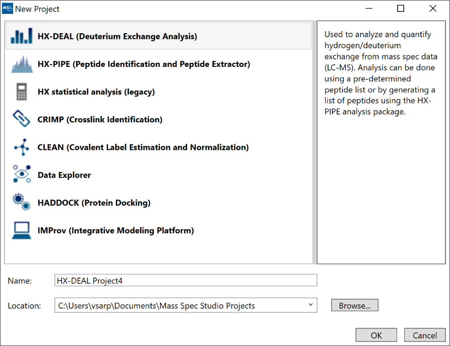
1. “New Project”: Create a new HX-DEAL project by selecting “New Project” and selecting “HX-DEAL”. The default location for new projects will be inside your home directory. You can select a different location by clicking “Browse” and selecting a new directory.
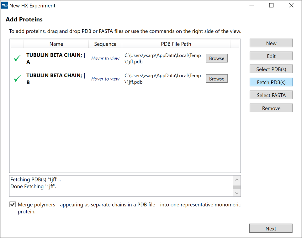
2. “Add Proteins”: If you have more than a single protein or
wish to use sequence visualizations, you can add your protein sequences either
manually (“New”), via a FASTA file (“Select FASTA”), via a PDB file (“Select
PDB(s)”), or via a 4-letter PDB code (“Fetch PDB(s)”, example: “1jff”). Each
protein will be listed as a separate row. If you have both PDB and FASTA, you
can add the FASTA file first and then use the “Browse” button to link the PDB
file. If you add both the PDB file and the FASTA file spearately, you may end up
with duplicate proteins in the table. Important: For the
sequence visualizations to work, the names of the proteins must match those
found in the Peptide .csv file (explained later).
The “Merge polymers” option can be used to remove duplicate sequences from
multimeric protein complexes which may appear as separate chains inside a PDB
file. Example PDB-code: “1fu1”.
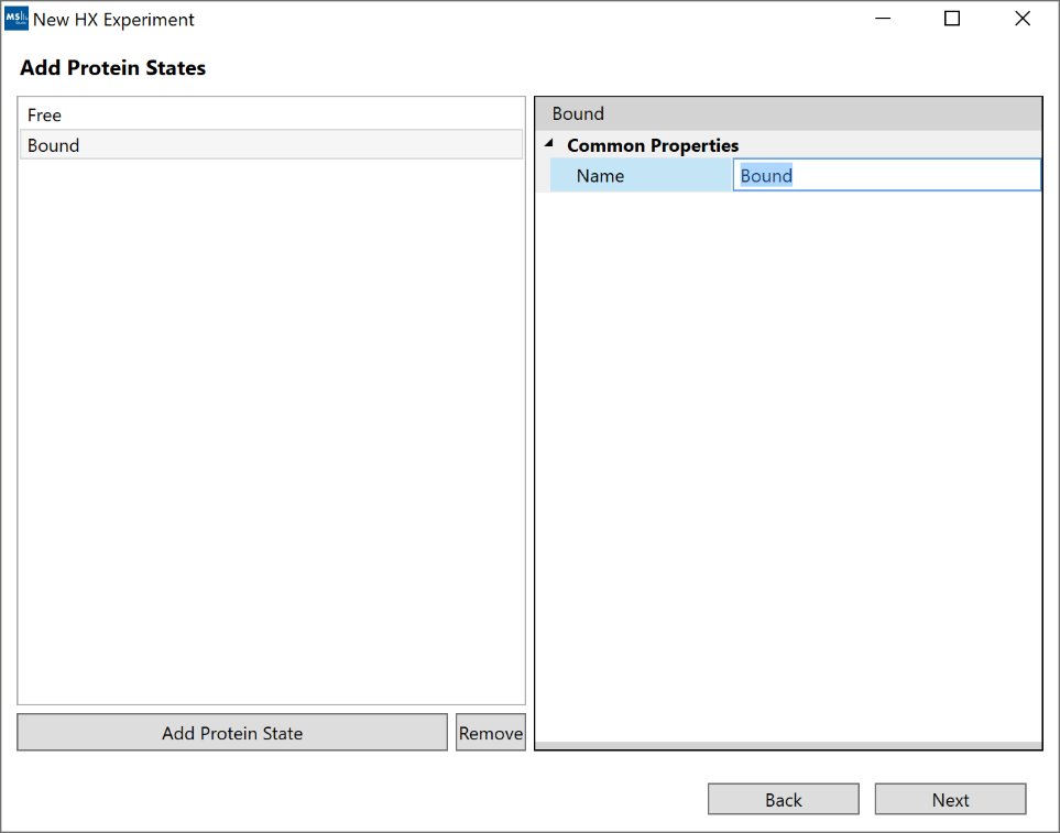
3. “Add Protein States”: For simple analysis, at least 1 protein state is required. For the additional comparative analysis tools and visualizations to become available, you must supply at least 2 proteins states.
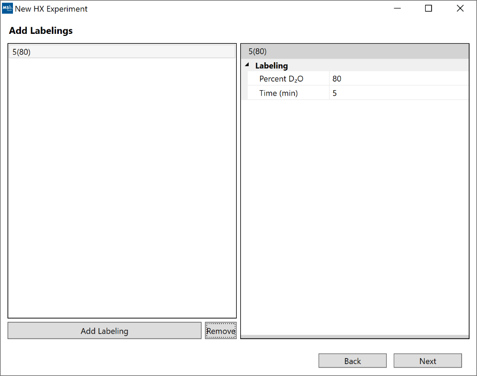
4. “Add Labeling”: At least 1 labeling condition is required (both time and %D2O). For kinetics visualizations to become available, you must supply at least 2 labeling conditions.
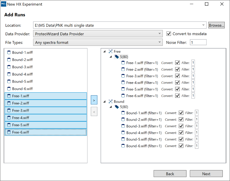
5. “Add Runs”: Follow these steps to add your data:
- a. Click “Browse” and select the root folder which contains your raw data files. In cases where the data files themselves are directories (example: Waters, Bruker), please make sure the containing folder is selected not the top-level .raw or .d directory itself. Note: Not all files have to be located under the same root folder from the start. After you add some files, you can still “Browse” to a different root directory and select additional files from the new location.
- b. For most raw vendor files, we recommend to use “ProteoWizard Data Provider”. If you have Mass Spec Studio converted files (.mssdata, .mssmeta), select “Mass Spec Studio Data Provider”.
- c. We recommend you enable the “Convert to mssdata” checkbox. When ON, raw vendor files will be converted to the .mssdata format which enables super-fast searching at the cost of some additional disk space for the .mssdata files. You can still proceed without converting the files, but the processing will be very slow. The “Noise filter” value is a multiplier of the minimum signal in each spectrum. A noise filter of “2” will remove any intensities smaller than 2 * mininum. A value of “0” will not remove any data.
- d. Select your replicates (shift+click or ctrl+click for multi-select), select the appropriate Protein State/Labeling node and click the “>” button. If you make mistakes, you can remove runs using the “<” button.
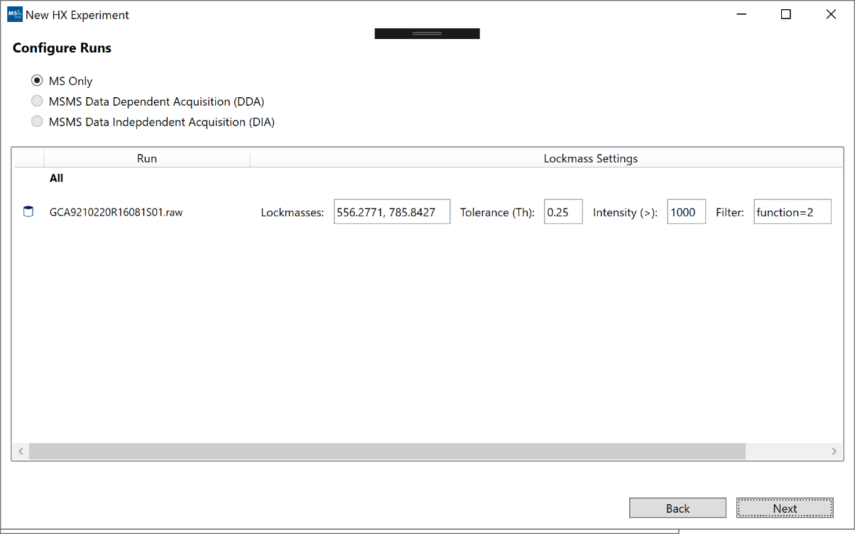
6. “Configure Runs”: For most files, no further action needed here. For Waters files, you will have the option to change the default lockmass settings. These settings will only be applied if the data is not already calibrated from ProteoWizard. The “Filter” settings will default to the last function in each data file. If your reference function is not the last function, you must provide the function number manually.
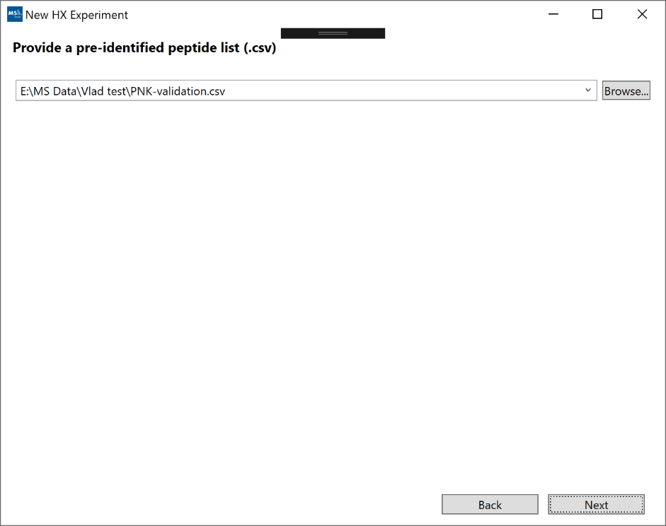
7. “Provide a pre-identified peptide list (.csv)”: Click “Browse” and select a peptide list. Note: To avoid duplicates, it’s recommended that your peptide identifications are grouped by sequence and charge such that each peptide (sequence/charge pair) has only one "RT". If you start with multiple separate peptide-specturm matches (PSMs) for the same peptide, you can group them by sequence/charge and average their RTs to get the final peptide "RT". Furthermore, you can use the optional "RT Variance" parameter to cover the full range of the original PSM RTs.
A sample peptide list: sample_peptides.csv
The list of currently supported headers (case-insensitive):
- “Protein” [required for sequence visualization]: The protein name. This should match the FASTA or PDB files for the visualizations to work. [alternatives: "ProteinSource", "protein.Accession", "prot_desc"]
- “Start” [required for sequence visualization]: The number of the first amino acid. [alternatives: "AminoAcidStart", "peptide.seqStart", "pep_start"]
- “Stop” [required for sequence visualization]: The number of the last amino acid. [alternatives: "End", "AminoAcidStop", "pep_end"]
- “Sequence” [required]: The peptide sequence. [alternatives: "peptide.seq", "pep_seq"]
- “Charge” [required]: The peptide charge. [alternatives "z", "precursor.z", "pep_exp_z"]
- “Monoisotopic Mass”: The peptide monoisotopic mass. If the monoisotopic mass is not supplied, it will be calculated from sequence, charge and modification composition. [alternatives: "m/z", "precursor.mz", "pep_exp_mz"]
- “Retention Time”: The average retention time of the peptide in minutes. If no RT is supplied, then the tallest XIC is selected by default. [alternatives: "RT", "RetentionTime", "precursor.retT"]
- “Retention Time Variance”: The one-side variance of the retention time in minutes. This range is used to search for the best fitting XIC peak. The fit is performed on the MS data. Default is 0.2min. [alternatives: "RTVariance", "RT Variance"]
- “Modification Composition”: The composition of any post-translational modification. Example, oxidation would be “O” or “O1”. [alternatives: "Modification Formula"]
- “Ion Mobility”: If using ion mobility, the peptide drift time in milliseconds. [alternatives: "Drift Time"]
- “Ion Mobility Tolerance”: If using ion mobility, the tolerance of the peptide drift time in milliseconds. [alternatives: "Drift Time Tolerance"]
- “Notes”: Any useful peptide-specific notes to be carried through analysis.
Note: Peptide .csv files from Waters PLGS are also supported.
8. Summary”: The summary screen will show a top-down view of the project setup. Any missed errors or hints will appear under each step. Clicking on a row in the summary table will navigate back to that section of the wizard.
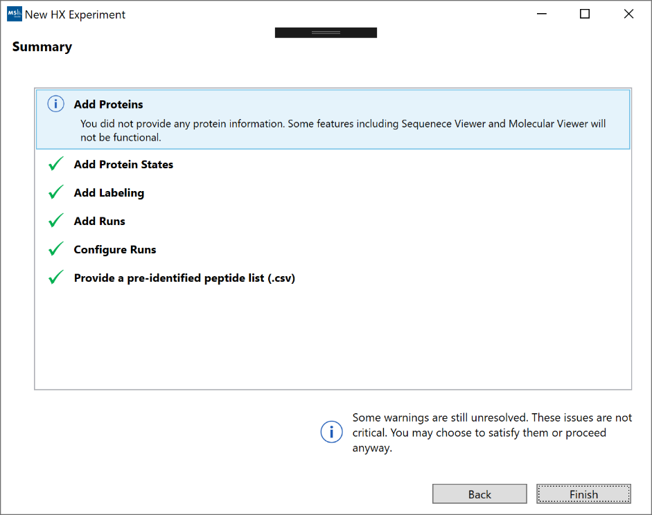
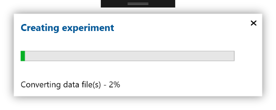
9. Complete the setup wizard by clicking “Finish”. A progress bar will appear to track the creation of the project:
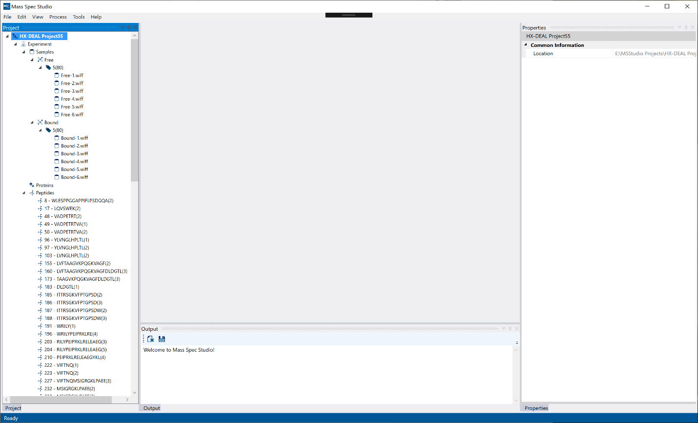
Project Structure
Once the HX-DEAL project is created, you will see an empty project view with an empty document section (middle) and left, bottom and right-side panels. The project tree structure will appear on the left panel with the protein states, labeling, runs, proteins, peptides, and results. The right panel will be a general “Properties” view where information from selected elements will appear (example: after processing, selecting a peptide will display the deuteration information on the Properties panel). The bottom panel will initially contain the “Output” for an empty project. Once processed, the peptide list will also appear on the bottom panel.
Hint: Panels and documents can be un-docked and moved to a different region or detached from the main window as a standalone window by clicking and dragging on the blue toolbar for panels and the title tab for documents. Clicking the pin icon will minimize a panel for a more compact view.
Hint: If any panels (left, right, bottom) are closed, they can be brought back from the “View” toolbar. To bring back the result views (middle - documents), you can double click on a result.
Processing
Once a project is created, you can open the processing window from the “Process” option on the main menu. The processing window has 3 areas:
- 1. The “Processing Routines” area will list the available routines that can be applied to your project. HX-DEAL has a single default “Peptide HX-MS” routine. Incompatible routines (for other project types) may appear in grey and can be hidden if the “Show Compatible Routines Only” checkbox is enabled.
- 2. The “Recent Parameters” area will save your most recent (last 5) parameter settings from previous successful runs.
- 3. The main right-side area will contain the list of adjustable parameters for the selected processing routine. Advanced users can choose to display additional “Advanced Parameters” from the checkbox on the top-right, which enable more control over the analysis. Parameters can be saved/loaded by interacting with the “Recent Parameters” list or to/from file (XML) via the “Open” and “Save” button on the bottom left./li>
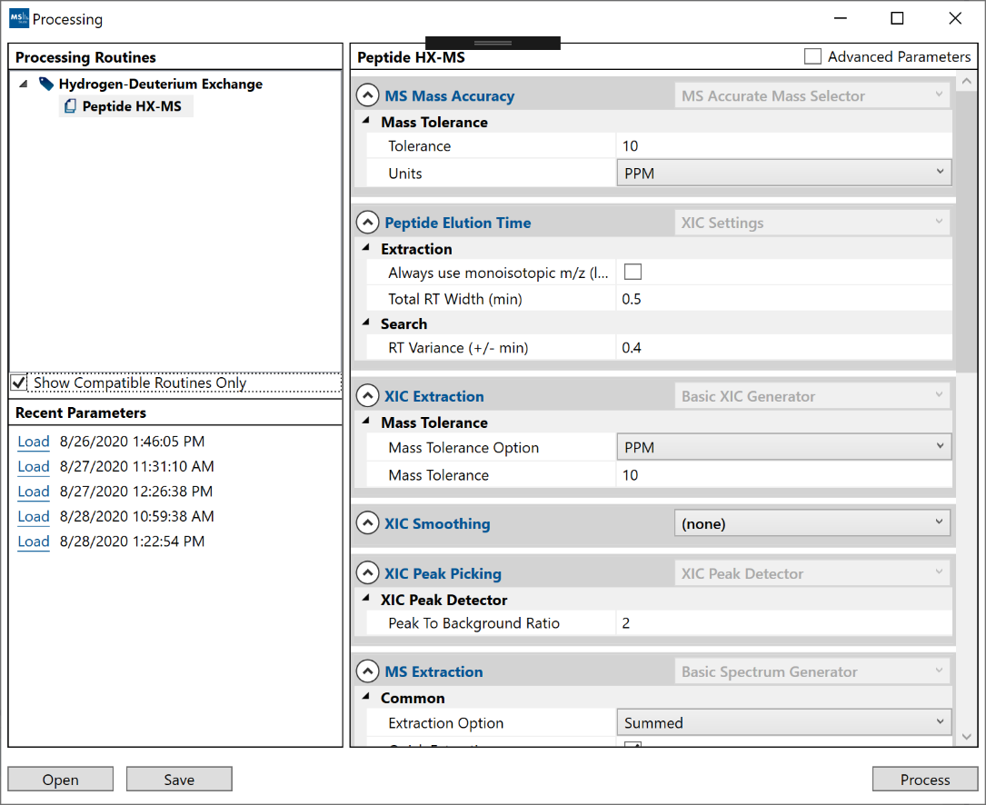
The search parameters for Peptide HX-MS analysis:
- “MS Mass Accuracy”: The mass tolerance when searching for MS peaks in the expected mass windows for the deuterated/non-deuterated isotopes of a given peptide. The tolerance is one-sided, meaning that a 10 ppm tolerance will span -10 ppm to the left and +10 ppm to the right of an expected peak.
- “Peptide Elution Time”: Settings for dealing with XIC data and
peptide retention times:
- “Always use monoisotopic m/z (lock)”: If enabled, the XIC is extracted around the monoisotopic peak instead of the most intense peak. Enabling this may cause heavier or highly-deuterated peptides to have poor XICs due to the monoisotopic peak having low intensity.
- “Total RT Width (min): The total elution time range of a peptide if not pre-set in the initial peptide list. A setting of 0.5 minutes will extract from RT-0.25min to RT+0.25min.
- “RT Variance (+/- min)”: The range around the expected RT of a peptide in which we look for good XIC peaks. This setting is one-sided such that a value of 0.4min will search for good XIC peaks from RT-0.4min to RT+0.4min.
- “XIC Extraction”: The m/z window used in extract the XIC for a given peptide. This setting is similar to the “MS Mass Accuracy” where the PPM value is one-sided. This mass range will be applied around the best peak or the monoisotopic peak for XIC extraction, depending on the “Always use monoisotopic m/z (lock)”.
- “XIC Smoothing”: The type of smoothing for the XIC.
- “XIC Peak Picking”: The settings for finding peaks in the XIC data.
- “MS Extraction”: The ranges for extracting MS data once the best RT range for the peptide is found. By default, it will extract a “Summed” spectrum using the defined RT range. The “m/z Padding” is the m/z range relative to the monoisotopic.
- “MS Smoothing”: The type of smoothing for the aggregated MS data.
- “MS Peak Picking”: The settings for finding peaks in the aggregated MS data.
- “Deuterated Profile Finder”: Settings to control automatic peak selection for the deuterated profile of a given peptide. Instead of using the number of peaks or strict m/z ranges, the Studio will attempt to pick peaks inside expected m/z windows only if they fit an expected pattern (EX2 by default). The “% Intensity Threshold” defines the % peak intensity relative to the most intense peak used in the automatic peak selection. The finder will pick consecutive peaks until a peak intensity falls below the threshold (unless there is an EX1-type pattern where there appear to be a fast and a slow exchanging profile for the same peptide). Note: Not all peaks need to be selected for the deuterium calculation, only enough good peaks to perform the standard EX2 binomial expansion or the double binomial expansion for suspected EX1 cases. Example: In a deuterated profile with 5 peaks, if 2 of the peaks are overlapped, the deuteration can still be calculated by fitting the remaining non-overlapped peaks.
- “Deconvolution Defaults”: Deconvolution (OFF by default) can help a user understand overlaps or scenarios where the peptide doesn’t fit a common EX2 expansion pattern. The frequencies from the non-deuterated peptide are removed from the frequencies of the observed MS spectrum in FFT space to give a better idea where the deuterons themselves are located. The “Centroid” option will use only the centroided peaks to do the FFT calculations, whereas the “Kaiser-Bessel” option will be applied on the raw intensities of the MS-spectrum.
- “Deuteration Results Generator”: Basic settings on how deuteration is calculated on the peptide. The “Number of Exchangers” setting allows the user to define whether the terminal amide is exchangeable. By default, the number of exchangers is set to be # of residues minus # of prolines minus 2 (N-p-2, where the terminal amide is not included).
- “Result Settings”: These settings control whether the raw MS and XIC data is saved in the result files. When the data is stored to file, the result will take up significantly more disk space but the interaction with the manual validation will be faster. When the option to save data to file is de-selected, the XIC and MS spectra will be generated live when clicking on a peptide which may lead to slower initial loading of peptides/replicates but faster project opening and smaller disk space usage for results. By default, all data is saved in the results file.
The default parameters should work for most runs. If you are seeing instances where good peaks are not selected by default, try widening the “MS Mass Accuracy” and “XIC Extraction” ranges.
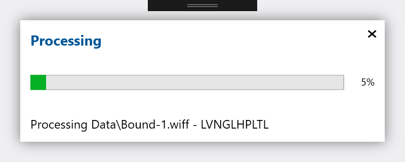
The processing routine will calculate deuteration for all your peptides across all your data file. When finished, a new result will appear in the “Results” section of your project tree. The processing routine can be re-run as many times as needed with different parameters combinations, with each result saved separately. Double-click on a result to open up the manual validation view as well as the rest of the visualizations in the middle document region.
Manual Validation
The manual validation view allows you to further refine and correct your results from the automatic analysis. Changes during manual validation will appear live on the visualizations for the selected result. Some examples of what you may want to do using the manual validation view:
- - Navigate and inspect each replicate by filtering Proteins State and Labeling (top toolbar).
- - Fix any missing or inaccurate peak selections.
- - Adjust RT ranges for aggregated MS extraction and XIC mass.
- - Change mass exchange regime for each replicate (EX1 vs default EX2 – “Is EX1” ON/OFF).
- - Remove peptides (across all replicates, states, labeling) if they are not found or too noisy.
The mass spec graph and XIC are interactive. To zoom in, click and drag on the X or Y axis. The mouse wheel will also zoom but on the X-axis only. Double clicking an axis will reset the zoom level to fit all of the data.
On the MS graph, the red line is the theoretical distribution of the unmodified peptide. The black line is the best fit of the selected peaks based on a binomial expansion of the exchangeable amides. Poor fits will be flagged in the replicates table and their p-value is displayed on the Properties panel. For scenarios where the poor fit is due to a EX1 exchange regime, selecting “Is EX1” will perform a double binomial fit and attempt to calculate the deuteration and population of each species (fast/slow exchange) separately.
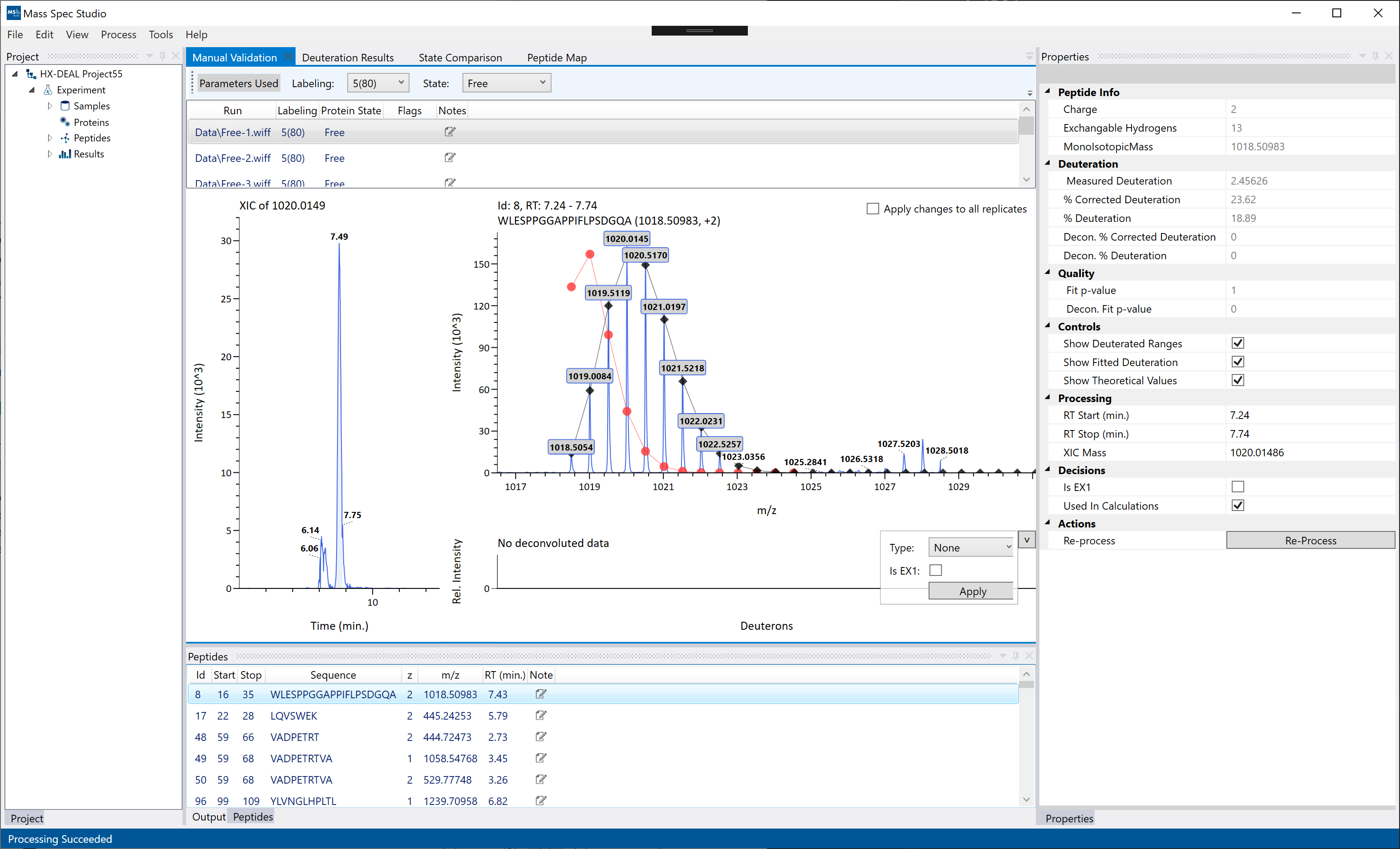
The replicate-level deuteration results are displayed on the right-side panel ("Properties") for the selected peptide in the Peptides table and the selected state/labeling pair in the Manual Validation table (top). Changes to peak selections will automatically update the deuteration values. If you wish to disable a single replicate without deleting an entire peptide, toggle the "Used in Calculations" flag. If "Used in Calculations" is diabled, then the deuteration value from that single replicate is ignored in broader visualizations and exports.
Hint: If you are adjusting peak selections manually, you can enable “Apply changes to all replicates” to mirror the same peak selections on the whole replicate set for the given Labeling + Protein State.
Hint: To remove an entire peptide from the dataset, you can right-click and delete it directly from the peptide list. Deleting a peptide will completely remove the peptide from ALL states/labeling/replicates for the current result. If you wish to exclude a single replicate, you can uncheck the “Used in Calculations” options in the properties panel.
Hint: The sections of the manual validation view are adjustable. Hovering your cursor between sections (ex: between MS and deconvolution section) will reveal a thin blue splitter which can be dragged to adjust the size of each section.
Visualizations
Most visualizations are customizable and exportable as high-res images. For most graphs like the MS graph, the XIC or the kinetics plots, you can right-click to bring up the image saving wizard. For more complex controls like the sequence coverage view or the peptide map, there will be a button on the toolbar to save images. Note: Visualizations can also be exported as a bundle via the File -> Export wizard (see Export section below).
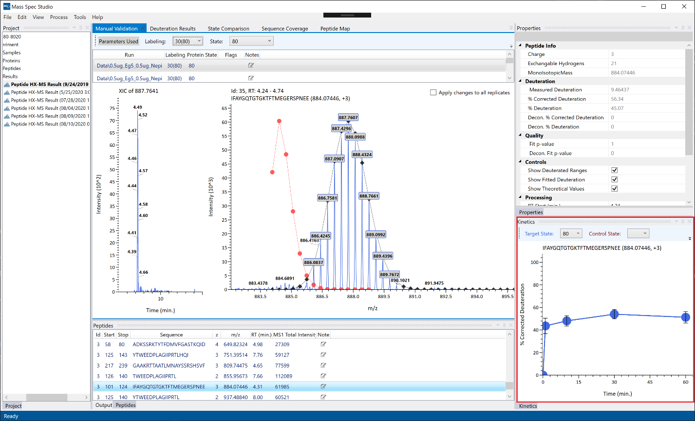
Kinetics: The kinetics view will appear on the bottom-right panel by default if the project contains more than one timepoint. To view the whole set of commands available on the toolbar (error bars, line thickness, bubble size), you can click on the small black arrow at the top right of the toolbar.
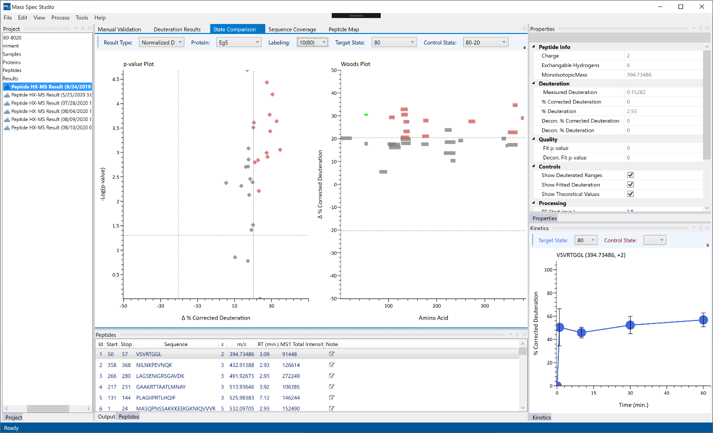
State Comparison: The state comparison view is available for any projects containing more than one protein state. For each combination of protein states, the deuteration difference for each peptide is calculated using a Students T-Test. The T-test deltas and p-values are plotted on the Volcano plot (left) and on the Woods Plot (right). Selecting a point or a sequence will navigate to the respective peptide on the peptide list.
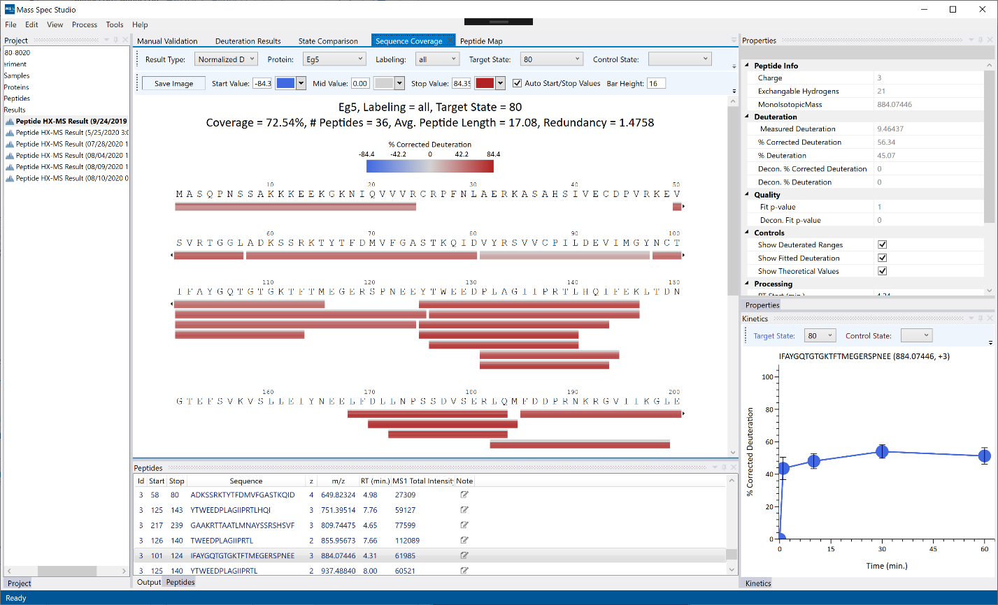
Sequence Coverage: Peptides are displayed as colored bars below their respective protein sequences. If “all” labeling is selected, the bars will show deuteration values for each replicate as a vertical gradient. If a single timepoint is selected, then the whole peptide bar will show the average deuteration for the replicate set for the given timepoint. To show the comparative view between 2 states, a Control State must be selected and the bars will display delta values instead.
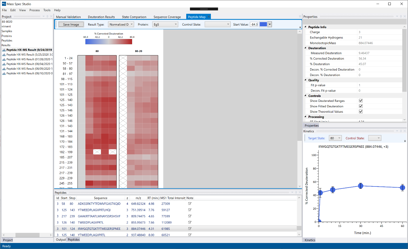
Peptide Map: The peptides are separated by Protein State and aggregated by start/stop and displayed on a grid with ascending time points from left to right. The color represents the average deuteration or the delta deuteration if a Control State is selected. An empty square (X) means that there is no data for that timepoint/state/peptide combination.
Export
To export a result, you can click on “File -> Export” and use the Export wizard to select and customize the data you wish to extract.
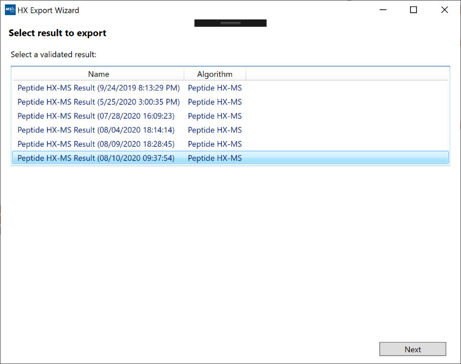
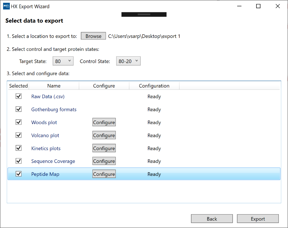
After selecting the result you wish to export, you can select the type of data and visualizations which should be included in the export bundle. If you have more than one protein state defined in your project, the default export mode will be a comparative analysis between two states. The list of export options (some may not be available, depending on project structure):
- “Raw Data”: A .csv file containing the results for each peptide.
- “Gothenburg formats”: The recommended HDX-MS publication format defined in https://www.ncbi.nlm.nih.gov/pmc/articles/PMC6614034/. This options will export a .csv file with deuteration values for all peptides as well as a experiment-level summary file.
- “Woods plot”: The Woods plot view as a .tiff image. [Requires configuration]
- “Volcano plot”: The Volcano plot view as a .tiff image. [Requires configuration]
- “Kinetics plots”: The kinetics plots for all peptides as .tiff images. [Requires configuration]
- “Sequence Coverage”: The sequence coverage view as a .tiff image. [Requires configuration]
- “Peptide Map”: The peptide map view as a .tiff image. [Requires configuration]
If you select any options which require manual configuration, you will need to click the “Configure” button before proceeding. For most options, a window ill pop up with a customizable template of what the image will look like prior to export. Once the configuration is complete for a given row, the status will change to “Ready” and any exported images for that option will use your custom settings.
Note: For projects with multiple proteins, the images will be grouped per-protein in the final export bundle.